Plotting the BSE fatband structure of Si
Task
Visualization of the BSE eigenvectors using fatbands.
Input
Si
 5.4300
0.5 0.5 0.0
0.0 0.5 0.5
0.5 0.0 0.5
2
cart
0.00 0.00 0.00
0.25 0.25 0.25
INCAR
- This is the INCAR file for the basic DFT calculation:
System  = Si

PREC = Normal ; ENCUT = 250.0

ISMEAR = 0 ; SIGMA = 0.01
KPAR = 2

EDIFF = 1.E-8
NBANDS = 16
LOPTICS = .TRUE.  # needed for WAVEDER file
LPEAD = .TRUE.
OMEGAMAX = 40
KPOINTS
The KPOINTS file will be automatically generated in this example.
Calculation
- In this example we will calculate and plot the first "bright" BSE eigenstates of silicon, also called fatbands[1]. In this tutorial the modelBSE setup from the previous tutorial is used in combination with a 10x10x10 gamma centered k-point grid (Note: This calculation takes ~ 50 min. on 16 cores, if you don't want to wait that long, a 4x4x4 grid requires only a minute.) In principle the standard BSE method can also be used instead.
Step 1 DFT calculation
We run a standard DFT calculation with the input files given above.
Step 2 BSE calculation with fatbands
- The INCAR file for the modelBSE calculation looks like the following:
System  = Si

PREC = Normal ; ENCUT = 250.0

#ALGO = BSE
ANTIRES = 0
ISMEAR = 0 ; SIGMA = 0.01
ENCUTGW = 150

EDIFF = 1.E-8 # default 1.E-4
NBANDS = 16   # only bands that are used are required, prepare the same set in a forgoing DFT run
NBANDSO = 4
NBANDSV = 8
OMEGAMAX = 20

PRECFOCK = Normal

ALGO = TDHF
LMODELHF = .TRUE. #Turn model on
HFSCREEN = 1.26  # Screening lenght
AEXX = 0.088    #Inverse of epsilon_infinity
SCISSOR = 0.69  # Difference GW-DFT band gap

NBSEEIG = 10 # number of BSE eigenvectors written out in BSEFATBAND
- The important tag for fatband calculations is NBSEEIG. In this example this will write the 10 energetically lowest BSE eigenvectors to the output file BSEFATBAND.
- After the (model)BSE calculation we first look into the vasprun.xml file to have a look at the BSE eigenvalues and the oscillator strengths (exact numbers can of course differ depending on the method you use and the density of your k-point grid):
<varray name="opticaltransitions" >
 <v>      3.148           0.000 </v>
 <v>      3.148           0.000 </v>
 <v>      3.148           0.000 </v>
 <v>      3.149       25654.244 </v>
 <v>      3.149       25660.601 </v>
 <v>      3.149       25665.652 </v>
 <v>      3.151           0.001 </v>
 <v>      3.151           0.001 </v>
 <v>      3.152         423.751 </v>
 <v>      3.310      216931.963 </v>
 <v>      3.310      216916.814 </v>
 <v>      3.310      216935.593 </v>
The first number column shows the BSE eigenvalue and the second one the oscillator strength. We are going to plot the first "bright" state, that means in this case number 4.
- We inspect the fourth band in the BSEFATBAND output file:
             28428                10
     1BSE eigenvalue    3.14798542      IP-eigenvalue:    3.25790292
  0.00000  0.00000  0.00000    -6.1302666     9.0994773       0.0000001     1     5     -0.000000+i*    -0.000000
  0.00000  0.00000  0.00000     5.8415744     9.0994773       0.0876503     2     5      0.000076+i*     0.000043
  0.00000  0.00000  0.00000     5.8415744     9.0994773     341.0850802     3     5      0.088630+i*    -0.329369
  0.00000  0.00000  0.00000     5.8415744     9.0994773     543.1678695     4     5      0.361803+i*    -0.405130
  0.00000  0.00000  0.00000    -6.1302666     9.0994773       0.0000004     1     6     -0.000000+i*     0.000000
…(28428-6 more lines till 2BSE eigenvalue …)
     4BSE eigenvalue    3.14855812      IP-eigenvalue:    3.25790292
  0.00000  0.00000  0.00000    -6.1302666     9.0994773       0.0024165     1     5      0.000002+i*     0.000001
  0.00000  0.00000  0.00000     5.8415744     9.0994773      31.4738813     2     5     -0.027821+i*    -0.014718
  0.00000  0.00000  0.00000     5.8415744     9.0994773     187.8684774     3     5      0.049093+i*    -0.181341
  0.00000  0.00000  0.00000     5.8415744     9.0994773     360.1697144     4     5      0.239775+i*    -0.268757
  0.00000  0.00000  0.00000    -6.1302666     9.0994773       0.0289534     1     6      0.000019+i*    -0.000022
...
The description of the values is given as follows:
- line: Number of e-h pairs in the BSE basis and value for NBSEEIG.
- line: BSE eigenvalue and minimum band gap before BSE.
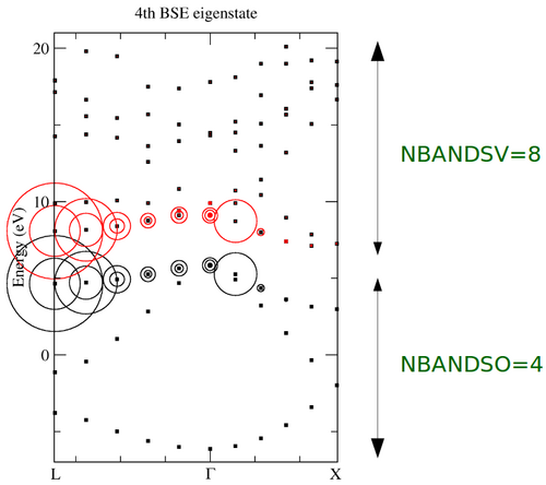
- line: Columns 1-3 k-point coordinates, column 4 hole eigenvalue, column 5 electron eigenvalue, column 6 absolute value of coupling coefficient (radius of circles), column 7 hole orbitalnumber, column 8 electron orbitalnumber, column 9 real part of coupling coefficient, column 10 imaginary part of coupling coefficient.
Columns 1-6 are used to plot the fatbands.
- Plotting of data:
- Choose the BSE eigenstate from the BSEFATBAND file that you want to plot.
- Filter out all e-h pairs that lie on the high symmetry k-lines along which you want to plot the fat bandstructure:
#!/bin/bash
NBSE=1 #Select the BSE eigenvector of interest.
BSIZE=$(head -n 1 BSEFATBAND|awk '{print $1}') # The BSE product basis size.
i=`echo "($BSIZE+1)*$NBSE+1"|bc`
head -n $i BSEFATBAND | tail -n $BSIZE > BSE-$NBSE.dat #Cut out the selected eigenstate.
awk <BSE-$NBSE.dat  ' { if ($1==$2 && $3==$2) print sqrt($1*$1+$2*$2+$3*$3), $4, $5, $6 }' >bands-GL.dat
awk <BSE-$NBSE.dat  ' { if ($1==$3 && $2==0.0) print sqrt($1*$1+$2*$2+$3*$3), $4, $5, $6 }' >bands-GX.dat
- Use a plotting program to plot the output in the following manner:
|k-point|   electron        hole          |A|
           eigenvalue    eigenvalue
    x          y1            y2         radius
- The sample output for this tutorial should look like the following:
The fat band picture allows you to visually inspect which e-h pairs contribute the most to a particular BSE eigenstate. When k-point convergence is important, you can use it to truncate your e-h product basisset by choosing smarter NBANDSO/NBANDSV and/or OMEGAMAX values. Try NBANDSO=NBANDSV=2and check how much this effects the BSE results.

