Nuclephile Substitution CH3Cl - BM

From VASP Wiki

Task

In this example the nucleophile substitution of a Cl- by another Cl- in CH3Cl is simulated using blue-moon sampling.

Input

POSCAR

In the blue-moon sampling method several POSCAR files are used for different values of the collective variable.

Click to show/POSCARs
BM - POSCAR1
 1.0
12.0 0.0 0.0
0.0 12.0 0.0
0.0 0.0 12.0
 C    H    Cl
 1 3 2
direct
0.5871322375157908 0.55301018027835513 0.67971406677139101
0.62447012741721697 0.62816585397463176 0.66438574150817353
0.61071464532701736 0.47956072579783432 0.64324619181721654
0.51527571900478364 0.5538828554036046 0.73866022152099475
0.44165342598948132 0.58799096227020642 0.55554878133597507
0.7183326999654791 0.52000018063420794 0.8193619682794645


BM - POSCAR2
 1.0
12.0 0.0 0.0
0.0 12.0 0.0
0.0 0.0 12.0
 C    H    Cl
 1 3 2
direct
0.5799711358435562 0.55476678237160515 0.67294569944761984
0.62447012741721697 0.62816585397463176 0.66438574150817353
0.61071464532701736 0.47956072579783432 0.64324619181721654
0.51527571900478364 0.5538828554036046 0.73866022152099475
0.44165342598948132 0.58799096227020642 0.55554878133597507
0.72173007151589497 0.51914707229594526 0.82294649849296753


BM - POSCAR3
 1.0
12.0 0.0 0.0
0.0 12.0 0.0
0.0 0.0 12.0
 C    H    Cl
 1 3 2
direct
0.5728100341713217 0.55652338446485516 0.66617733212384878
0.62447012741721697 0.62816585397463176 0.66438574150817353
0.61071464532701736 0.47956072579783432 0.64324619181721654
0.51527571900478364 0.5538828554036046 0.73866022152099475
0.44165342598948132 0.58799096227020642 0.55554878133597507
0.72512744306631094 0.51829396395768246 0.82653102870647066


BM - POSCAR4
 1.0
12.0 0.0 0.0
0.0 12.0 0.0
0.0 0.0 12.0
 C    H    Cl
 1 3 2
direct
0.59507047500290222 0.57244270557313315 0.66746206851391643
0.54049944202575662 0.60714565557876798 0.72974089156310651
0.66455173208019991 0.53195474180779956 0.70393149950062939
0.55747027889637368 0.53034945501598485 0.59848340437508063
0.65618532162250798 0.69708568471255838 0.57638613391759708
0.5000409863126819 0.4022456289304116 0.80922741395305486


BM - POSCAR5
 1.0
12.0 0.0 0.0
0.0 12.0 0.0
0.0 0.0 12.0
 C    H    Cl
 1 3 2
direct
0.59887853190304419 0.57974515358235179 0.6617842250921081
0.54049944202575662 0.60714565557876798 0.72974089156310651
0.66455173208019991 0.53195474180779956 0.70393149950062939
0.55747027889637368 0.53034945501598485 0.59848340437508063
0.65618532162250798 0.69708568471255838 0.57638613391759708
0.4980707241384853 0.3987068989373313 0.8121665955404771


BM - POSCAR6
 1.0
12.0 0.0 0.0
0.0 12.0 0.0
0.0 0.0 12.0
 C    H    Cl
 1 3 2
direct
0.60268658880318615 0.58704760159157043 0.65610638167029967
0.54049944202575662 0.60714565557876798 0.72974089156310651
0.66455173208019991 0.53195474180779956 0.70393149950062939
0.55747027889637368 0.53034945501598485 0.59848340437508063
0.65618532162250798 0.69708568471255838 0.57638613391759708
0.4961004619642887 0.395168168944251 0.81510577712789944


BM - POSCAR7
 1.0
12.0 0.0 0.0
0.0 12.0 0.0
0.0 0.0 12.0
 C    H    Cl
 1 3 2
direct
0.60649464570332823 0.59435004960078897 0.65042853824849134
0.54049944202575662 0.60714565557876798 0.72974089156310651
0.66455173208019991 0.53195474180779956 0.70393149950062939
0.55747027889637368 0.53034945501598485 0.59848340437508063
0.65618532162250798 0.69708568471255838 0.57638613391759708
0.4941301997900921 0.39162943895117058 0.81804495871532179

KPOINTS

Automatic
 0
Gamma
 1  1  1
 0. 0. 0.
  • For isolated atoms and molecules interactions between periodic images are negligible (in sufficiently large cells) hence no Brillouin zone sampling is necessary.

INCAR

PREC=Low
EDIFF=1e-6
LWAVE=.FALSE.
LCHARG=.FALSE.
NELECT=22
NELMIN=4
LREAL=.FALSE.
ALGO=VeryFast
ISMEAR=-1
SIGMA=0.0516
   
############################# MD setting ##################################
IBRION=0                                 # MD simulation
NSW=1000                                 # number of steps
POTIM=1                                  # integration step
TEBEG=600                                # simulation temperature
MDALGO=11                                # Andersen thermostat
ANDERSEN_PROB=0.10                       # collision probability
LBLUEOUT=.TRUE.                          # write down output needed to 
                                         # compute free-energy gradient
##############################################################################


  • The setting LBLUEOUT=.TRUE. tells VASP to write out the information needed for the computation of free energies.

Calculation

In the blue-moon sampling, the free energy difference is computed by integration of the free energy gradients computed for several points differing in the value of the collective variable distributed between known inital and final states. The gradients for each point are computed within a constrained molecular dynamics simulation (note the value of STATUS=0 for the collective variable defined in the ICONST file).

Running the calculation

The mass for hydrogen in this example is set 3.016 a.u. corresponding to the tritium isotope. This way larger timesteps can be chosen for the MD (note that the free energy is independent of the masses of atoms). The simulation for each of the points along the reaction coordinate is performed in a separate directory called 1, 2, ..., 7. These are created automatically by the run script. For practical reasons, we split our (presumably long) blue-moon calculation into shorter runs of length of 1000 fs (NSW=1000; POTIM=1). This is done automatically in the script run which looks as follows:

#!/bin/bash

drct=$(pwd)

runvasp="mpirun -np x executable_path"

# ensure that this sequence of MD runs is reproducible - not needed
# in a real-world application
rseed="RANDOM_SEED =         311137787                0                0"

#c loop over "points" (i.e. structures 
#c with difference value of CV)
for j in 1 2 3 4 5 6 7
do
  cd $drct
  mkdir ${j}
  cp POSCAR.$j ${j}/POSCAR
  cp POTCAR KPOINTS ICONST $j
  cd $j

  #c here we perform sequence of MD runs
  #c for each point 
  step=1
  while [ $step -le 7 ]
  do
    if ! test -f report.${step}
    then

      # ensure that this sequence of MD runs is reproducible
      cp ${drct}/INCAR .
      echo $rseed >> INCAR

      cp POSCAR POSCAR.$step
      $runvasp

      # ensure that this sequence of MD runs is reproducible
      rseed=$(grep RANDOM_SEED REPORT |tail -1)

      #c backup some important files
      cp CONTCAR POSCAR
      cp REPORT report.$step
      grep F OSZICAR > osz.$step
      cp vasprun.xml vasprun.xml.$step
    fi
    let step=step+1
  done
done

Free-energy profile

The free energy gradient is obtained as a ratio of two averages (see Constrained molecular dynamics). This is done by the script fgradBM.sh, which writes the free energy gradient vs. the collective variable to the file grad.dat:

Click to show/fgradBM.sh
#!/bin/bash

#c equilibration period
equil=2000

if [ -f "grad.dat" ]; then
   rm grad.dat
fi

touch grad.dat

for i in  1 2 3 4 5 6 7
do
  rm rep.*
  j=1
  while [ $j -le 100 ]
  do
    if test -f $i/report.$j
    then
      grep b_m $i/report.$j >> rep.$i.1
    fi
    let j=j+1
  done

  #c obtain ingredients for FE-gradfient calculation
  #c (cf. eq. 12 in JPCM 20, 064211 (2008))
  if test -f $i/report.1
  then
    #c value of the constrained coordinate
    x1=$(grep cc $i/report.1|head -1|awk '{print $3}')

    nlines=$(wc -l rep.$i.1|awk '{print $1}')
    let prod=nlines-equil

    #c calculation of the FE-gradfient 
    #c (cf. eq. 12 in JPCM 20, 064211 (2008))
    zet=$(grep b_m rep.$i.1|tail -$prod |awk 'BEGIN {a=0.} {a+=$3} END {print a/NR}')

    g1=$(grep b_m rep.$i.1|tail -$prod |awk 'BEGIN {a=0.} {a+=$5} END {print a/NR/"'${zet}'"}')

    echo $x1 $g1 >> grad.dat
  fi

done

To execute that script type:

bash ./fgradBM.sh

For our purposes, a simple trapezoidal rule can be used for the integration of gradients. For accurate calculations, more sohpisticated integration schemes should be considered. The free energy vs. collective variable is obtained by forward integration using the script integrateForward.py:

Click to show/integrateForward.py
#!/usr/bin/python

import string
import sys

f=sys.argv[1]

f=open(f,'r')

r=[]
g=[]

for line in f.readlines():
  line=string.split(line)
  num=len(line)
  if len(line)==2:
    r.append(float(line[0]))
    g.append(float(line[1]))

f.close()

tg=0.0
print r[0],tg
for i in range(1,len(r)):
  gg=0.5*(r[i]-r[i-1])*(g[i]+g[i-1])
  tg+=gg
  print r[i],tg

To execute that script type and write to the file free_energy.dat:

python integrateForward.py grad.dat > free_energy.dat

Finally to plot that file type:

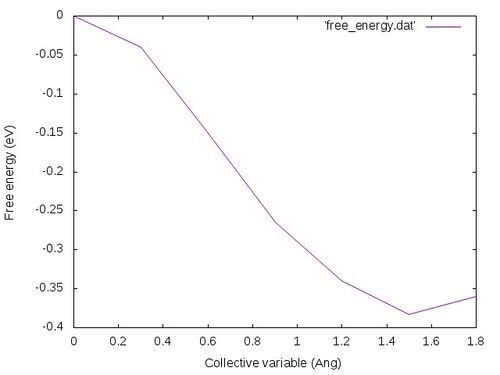
gnuplot -e "set terminal jpeg; set xlabel 'Collective variable (Ang)'; set ylabel 'Free energy (eV)'; set style data lines; plot 'free_energy.dat'" > free_energy.jpg

The free energy profile should look like the following:

Note that much longer simulations should be performed (typically a few tens or hundreds of ps) in order to achieve well converged averages needed in accurate calculations.

Download

CH3Cl_BM.tgz